
What is Joint Probability Model?
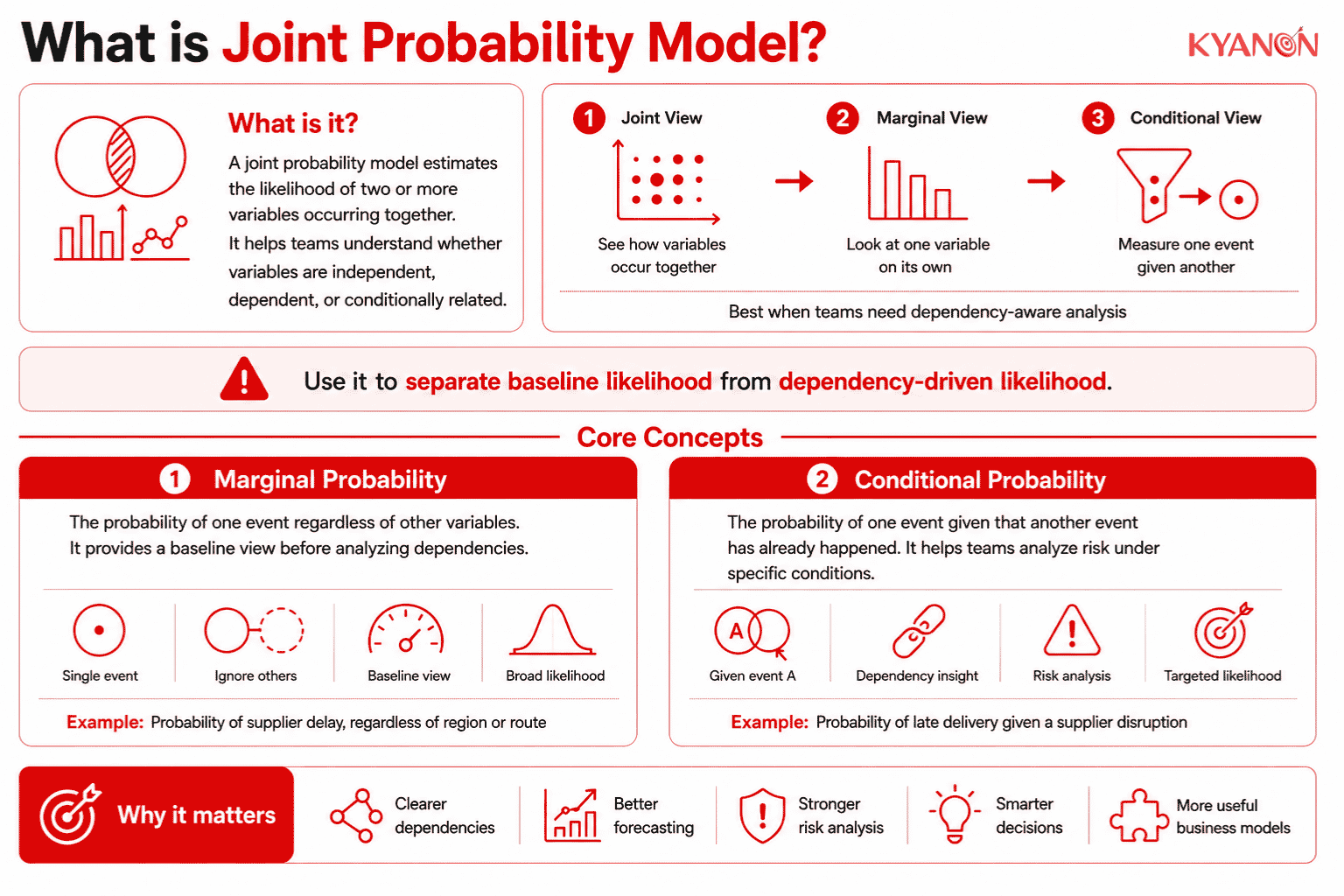
A joint probability model is a statistical framework that estimates the likelihood of two or more variables occurring together within the same data space. It is used to understand whether business variables are independent, dependent, or conditionally related.
Related Concepts in Joint Probability Model
A complete joint probability model can be analyzed through marginal probability and conditional probability, which describe different views of the same probability space. These concepts help business teams separate isolated likelihood from dependency-based likelihood.
Marginal Probability
Marginal probability is the probability of a single event occurring regardless of the other variables in the model. It is calculated by summing or integrating across the outcomes of the variables being ignored.
For example, a business may calculate the probability of supplier delay regardless of product category, region, or logistics route. This provides a baseline before analyzing how other factors change the probability.
Conditional Probability
Conditional probability is the probability of an event occurring given that another event has already happened. It is commonly written as: [P(B|A)]
For example, a planning team may estimate the probability of late delivery given that a supplier disruption has already occurred. This helps teams move from simple frequency tracking to dependency-aware risk analysis.

Discrete vs Continuous Joint Probability Models
Joint probability models adapt based on whether the data is countable or continuous. Discrete models use probability mass functions, while continuous models use probability density functions.
Joint Probability Mass Function
A joint probability mass function, or joint PMF, is used for distinct and countable outcomes. It can be represented in a joint probability table where each cell shows the probability of a specific combination of outcomes.
For example, a business may model the probability that a customer buys exactly two units of Product A and one unit of Product B. This is suitable for categorical, binary, or count-based business data.
Joint Probability Density Function
A joint probability density function, or joint PDF, is used for continuous variables with many possible values. Instead of assigning probability to one exact point, it measures probability across a range using the area or volume under a probability curve.
For example, a risk team may model the joint distribution of rainfall volume and wind speed to estimate severe weather disruption risk. This is useful when the variables are measured on continuous scales.
How Joint Probability Model Works
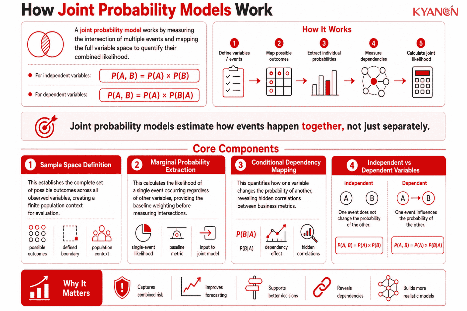
The model functions by determining the intersection of multiple events, mapping out the entire variable space to quantify their combined likelihood.
- For completely independent variables, it multiplies individual probabilities: $P(A, B) = P(A) \times P(B)$.
- For interdependent variables, it relies on conditional probabilities to measure how the presence of one variable alters the statistical likelihood of another: $P(A, B) = P(A) \times P(B|A)$.
Sample Space Definition
Establishes the complete set of possible outcomes across all observed variables. This boundary ensures the model evaluates probabilities against a finite, defined population context.
Marginal Probability Extraction
Calculates the likelihood of a single event occurring regardless of other variables. This baseline metric is required to establish the individual weighting of factors before measuring their intersection.
Conditional Dependency Mapping
Quantifies how the occurrence of one specific variable changes the statistical probability of another. This component exposes the hidden correlations between seemingly disconnected business metrics.
Frameworks for Structural Modeling
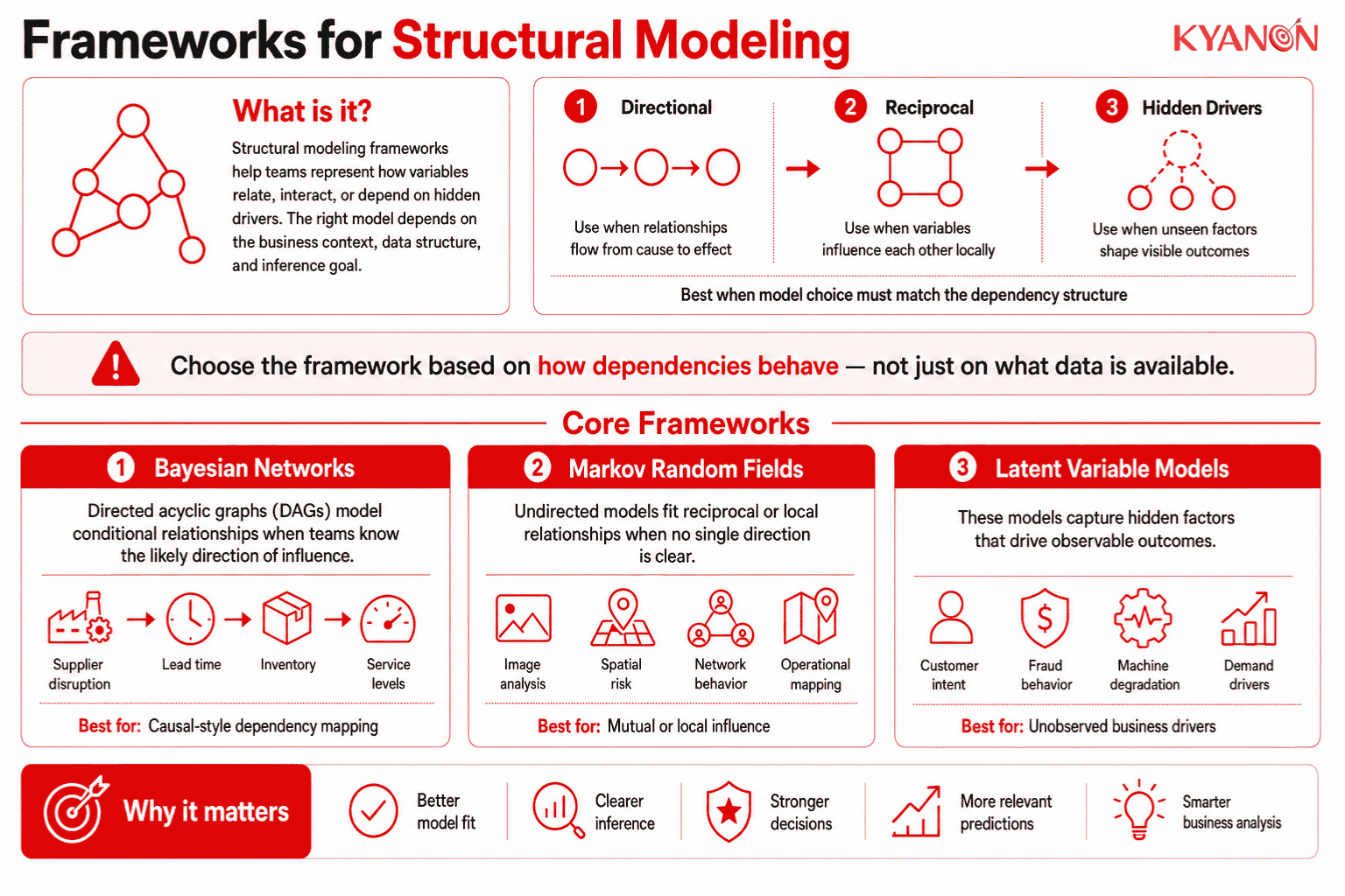
Different joint probability frameworks are used depending on whether dependencies are directional, reciprocal, or driven by hidden variables. The right framework depends on the business context, data structure, and inference goal.
Bayesian Networks
Bayesian networks use directed acyclic graphs, or DAGs, to represent conditional relationships between variables. They are useful when teams have domain knowledge about directional relationships, such as supplier disruption influencing lead time, lead time influencing inventory availability, and inventory availability influencing service levels.
Markov Random Fields
Markov Random Fields are undirected graphical models used when relationships are reciprocal or difficult to assign a strict direction. They are useful in systems where related variables influence one another locally, such as image analysis, spatial risk modeling, network behavior, or operational dependency mapping.
Latent Variable Models
Latent variable models are used when hidden factors influence visible outcomes. In enterprise analytics, this can apply to customer intent, fraud behavior, machine degradation, medical risk, speech recognition, or demand drivers that cannot be directly observed.
Real-World Applications
Joint probability modeling is used when business decisions depend on multiple events occurring together. It is especially relevant in finance, weather forecasting, machine learning, supply chain planning, risk analytics, and operational forecasting.
Finance and Investing
Finance teams can use joint probability modeling to estimate the likelihood that a specific asset declines while the broader market also moves downward. This helps risk teams understand portfolio exposure under combined market conditions.
Weather and Climate Risk
Weather forecasting teams can use joint probability models to estimate the simultaneous likelihood of freezing temperatures and high precipitation. This helps organizations prepare for events such as snowstorms, route disruptions, or infrastructure risk.
Machine Learning
Machine learning systems can use joint probability models to learn how data features and target outcomes interact. This is especially relevant in generative modeling, Bayesian inference, uncertainty quantification, and probabilistic classification.
Joint Probability Model vs Marginal Probability Model
Both approaches measure statistical likelihood but differ fundamentally in how they process multidimensional data dependencies.
| Dimension | joint probability model | Conditional Probability Model |
| Core question | How likely are A and B together? | How likely is A given B? |
| Formula | $P(A, B)$ | $P(A |
| Sample space | Full population or full data space | Restricted to cases where B has occurred |
| Best for | Modeling combined business scenarios | Estimating likelihood after a known condition |
| Example | Probability of high demand and delayed supply | Probability of delay given supplier disruption |
When to Consider Joint Probability Model
Consider joint probability model if:
- Your team needs to understand how multiple business variables interact, such as demand, pricing, customer behavior, supplier reliability, financial exposure, operational capacity, or fraud risk.
- Your AI roadmap includes Bayesian inference, probabilistic forecasting, anomaly detection, risk scoring, uncertainty quantification, or generative modeling.
- Your business decisions depend on combined events, such as high demand plus low inventory, delayed supply plus logistics congestion, unusual payment behavior plus fraud risk, or market volatility plus margin pressure.
It may not be the right priority if:
- Your current analytics use case only needs a simple single-variable metric, such as total revenue, shipment volume, monthly traffic, average order value, or total incidents. In that case, data quality, event tracking, and dashboard governance may matter more.
Why Joint Probability Models Matter for Supply Chain and Demand Planning
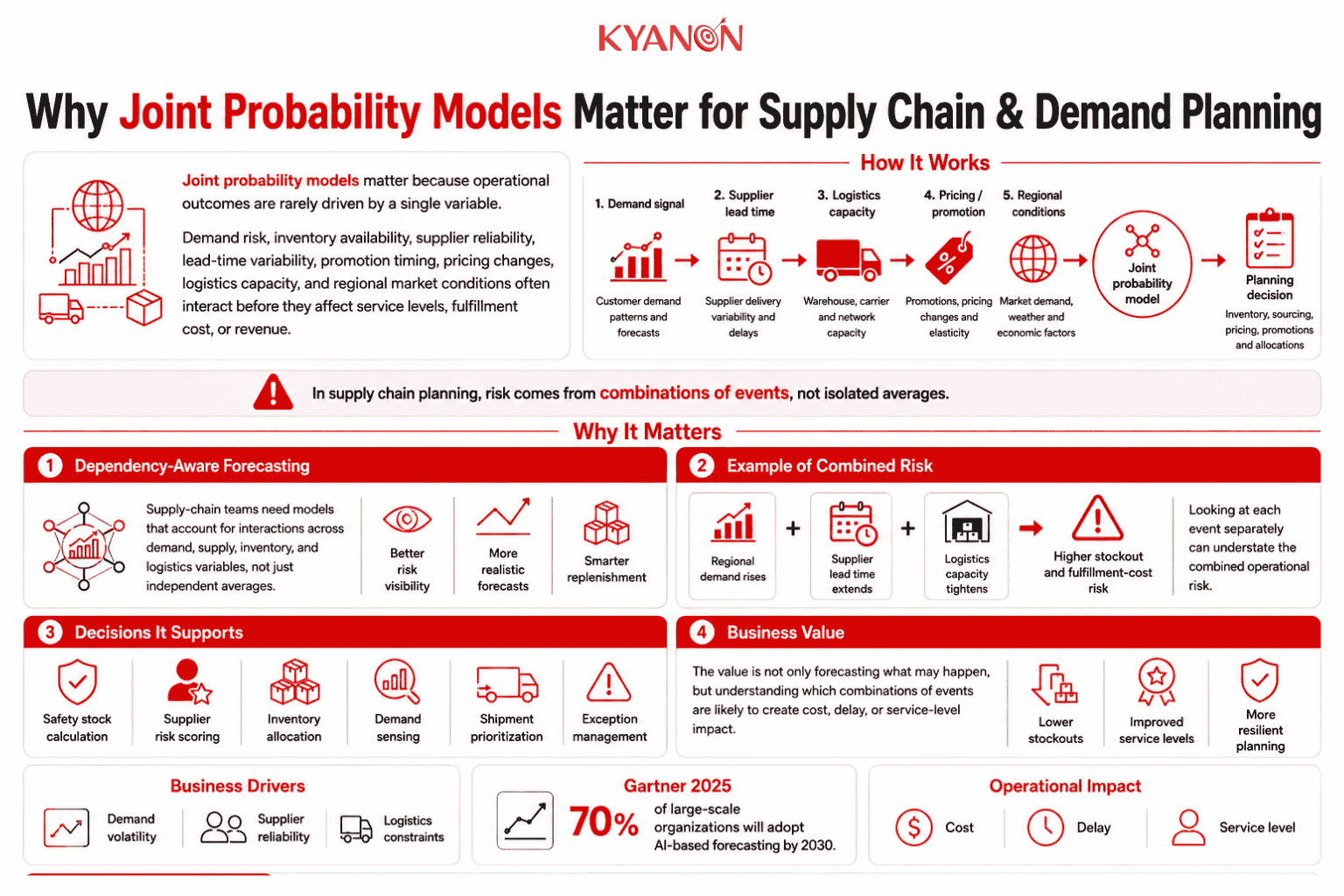
Joint probability models matter for supply chain and demand planning because operational outcomes are rarely driven by a single variable. Demand risk, inventory availability, supplier reliability, lead time variability, promotion timing, pricing changes, logistics capacity, and regional market conditions often interact before they affect service levels, fulfillment cost, or revenue.
Gartner predicted in 2025 that 70% of large-scale organizations will adopt AI-based forecasting to predict future demand by 2030. This makes dependency-aware probability modeling more relevant for supply chain teams because demand forecasts, replenishment plans, and risk signals depend on interacting business variables, not isolated averages.
For example, a distributor may need to estimate the probability that demand rises in one region while supplier lead times extend and logistics capacity tightens. Looking at each event separately can understate the combined operational risk, while a joint probability model evaluates the likelihood of those events occurring together.
In supply chain and demand planning, joint probability models can support decisions such as safety stock calculation, supplier risk scoring, inventory allocation, demand sensing, shipment prioritization, and exception management. The business value is not only forecasting what may happen, but understanding which combinations of events are likely to create cost, delay, or service-level impact.
Common Misconceptions
A common executive misconception is that joint probability modeling automatically means variables are independent, but joint models are often used precisely because variables may depend on one another.
“Joint probability means the events are independent.”
Reality: Joint probability does not mean the events are independent. Independence is only a special case where (P(A, B) = P(A) \times P(B)); when variables influence one another, the model must use conditional probability, such as (P(A, B) = P(A) \times P(B|A)).
“Joint probability equals conditional probability.”
Reality: Joint probability evaluates the likelihood of two or more events happening together across the total population. Conditional probability calculates the likelihood of one event only within the restricted sample space where another event has already happened.
“Joint probability implies causation.”
Reality: Joint probability measures statistical co-occurrence, not direct causation. Two events might frequently occur together because of an unmeasured confounding factor, shared seasonality, campaign timing, or coincidence.
“A full joint model is always the best machine learning approach.”
Reality: Full joint probability models can become expensive to train and maintain as the number of variables grows. Many enterprise systems use factorized, autoregressive, or discriminative approaches to balance model quality, data availability, latency, and implementation cost.
“Mutually exclusive events can have a joint probability above zero.”
Reality: Mutually exclusive events cannot happen at the same time, so their joint probability is zero. For example, a final payment decision cannot be both approved and declined in the same decision state.
How Kyanon Digital Applies Joint Probability Model
Kyanon Digital applies joint probability modeling in advanced analytics engagements where enterprise clients need to understand how business variables influence one another across customer, product, transaction, operational, financial, and risk data.
In projects across Vietnam, Singapore, Malaysia, Thailand, ANZ, the US, and Nordic Europe, this can support use cases such as demand forecasting, supplier risk analysis, fraud detection, pricing response analysis, predictive maintenance, and uncertainty-aware decisioning.
→ Explore our data and AI consulting services for enterprise probability modeling.

 Create project brief with AI